
More Information
Submitted: January 19, 2026 | Approved: January 28, 2026 | Published: January 29, 2026
How to cite this article: Sridhar LN. Analysis and Control of a Glucose-insulin Dynamic Model. Ann Clin Endocrinol Metabol. 2026; 10(1): 010-019. Available from:
https://dx.doi.org/10.29328/journal.acem.1001033.
DOI: 10.29328/journal.acem.1001033
Copyright License: © 2026 Sridhar LN. This is an open access article distributed under the Creative Commons Attribution License, which permits unrestricted use, distribution, and reproduction in any medium, provided the original work is properly cited.
Keywords: Bifurcation; Optimization; Control; Insulin; Glucose

Analysis and Control of a Glucose-insulin Dynamic Model
Lakshmi N Sridhar*
Chemical Engineering Department, University of Puerto Rico, Mayaguez, PR 00681, Puerto Rico
*Address for Correspondence: Lakshmi N Sridhar, Chemical Engineering Department, University of Puerto Rico, Mayaguez, PR 00681, Puerto Rico, Email: [email protected]
The dynamics of the glucose-insulin regulatory system are highly nonlinear and must be understood to be controlled effectively. Bifurcation analysis and multiobjective nonlinear model predictive control (MNLMPC) are performed on a glucose-insulin dynamic model. MATCONT was used for the bifurcation analysis, and for the MNLMPC calculations, the optimization language PYOMO is used in conjunction with the solvers IPOPT and BARON. The bifurcation analysis revealed a Hopf bifurcation point and a limit point. A Hopf bifurcation point is a tipping point where a system that was behaving steadily suddenly starts to oscillate or cycle on its own, like a machine that begins to vibrate instead of staying still. A limit point is a tipping point at which pushing a system a little further suddenly causes it to jump to a completely different state, rather than changing smoothly. MNLMC converged on the Utopia solution. The Hopf bifurcation point, which leads to an unwanted limit cycle, is eliminated by an activation factor. A limit cycle is a repeating pattern of behavior that a system naturally settles into over time, like a steady heartbeat or a clock that keeps ticking. The limit point (which causes multiple steady-state solutions from a singular point enables the Multiobjective nonlinear model predictive control calculations to converge to the Utopia point (the best possible solution) in the model. A Utopia solution in multi-objective nonlinear model predictive control is an ideal operating point at which all goals are simultaneously perfectly optimized.
Glucose–insulin dynamics describe the tightly regulated physiological processes that maintain blood glucose levels within a narrow range, ensuring a continuous supply of energy to tissues while preventing the harmful effects of hyperglycemia or hypoglycemia. This regulatory system involves complex interactions between glucose absorption, insulin secretion, tissue uptake, hepatic glucose production, and hormonal feedback mechanisms. Understanding glucose–insulin dynamics is fundamental in physiology, medicine, and systems biology, particularly in the study of metabolic disorders such as diabetes mellitus.
After a meal, carbohydrates are digested into glucose, which enters the bloodstream and raises plasma glucose concentration. Specialized β-cells in the pancreatic islets of Langerhans detect this increase via glucose metabolism and membrane depolarization. In response, insulin is secreted in a biphasic manner: an initial rapid release of pre-stored insulin followed by a slower, sustained phase driven by new insulin synthesis. This dynamic secretion pattern is crucial for limiting postprandial glucose excursions.
Insulin is the primary anabolic hormone that regulates glucose homeostasis. It promotes glucose uptake in insulin-sensitive tissues, particularly skeletal muscle and adipose tissue, by stimulating the translocation of glucose transporter type 4 (GLUT4) to the cell membrane. In the liver, insulin suppresses hepatic glucose production by inhibiting gluconeogenesis and glycogenolysis, while simultaneously promoting glycogen synthesis. These combined actions reduce circulating glucose levels and facilitate energy storage.
During fasting or between meals, insulin levels decline, and counter-regulatory hormones such as glucagon, cortisol, growth hormone, and catecholamines become more influential. Glucagon, secreted by pancreatic α-cells, stimulates hepatic glucose output to maintain adequate plasma glucose levels for glucose-dependent organs, especially the brain. The dynamic balance between insulin and these counter-regulatory hormones ensures metabolic stability under varying nutritional and physiological conditions.
Mathematical and computational models have been widely used to study glucose–insulin dynamics and quantify insulin sensitivity and β-cell function. Classic models, such as the minimal model of glucose kinetics, describe glucose-insulin interactions using coupled differential equations. These models capture essential features such as insulin-mediated glucose disposal and endogenous glucose production, providing valuable insights for both clinical assessment and control-oriented applications, including artificial pancreas systems.
Disruptions in glucose–insulin dynamics underlie metabolic diseases. In type 1 diabetes, autoimmune destruction of β-cells leads to absolute insulin deficiency, resulting in uncontrolled hyperglycemia. In type 2 diabetes, insulin resistance in peripheral tissues combined with impaired insulin secretion leads to chronic dysregulation of glucose levels. Over time, persistent hyperglycemia contributes to vascular, renal, neurological, and cardiovascular complications.
Glucose–insulin dynamics represent a highly coordinated, nonlinear control system that integrates hormonal signaling, tissue-specific responses, and feedback regulation. Their study provides a unifying framework for understanding normal metabolic function, disease mechanisms, and the development of therapeutic and control strategies to restore glucose homeostasis. Topp, et al. [1] developed a model of B-cells, insulin, and glucose that includes pathways to diabetes. Lenbury, et al. [2] modelled insulin kinetics, investigating responses to a single oral glucose administration or ambulatory-fed conditions. Shanik, et al. [3] investigated the relationship between insulin resistance and hyperinsulinemia. Han, et al. [4] developed a mathematical model of the glucose–insulin regulatory system from the bursting electrical activity in pancreatic β-cells to the glucose dynamics in the whole body. Lombarte, et al. [5] developed a mathematical model of glucose–insulin homeostasis in healthy rats. Boutayeb, et al. [6] conducted a mathematical modelling and simulation study of B-cell mass, insulin, and glucose dynamics, examining the effects of genetic predisposition to diabetes. Ho, et al. [7] provided insulin-sensitivity predictions for individuals with obesity and type II diabetes mellitus using a mathematical model of the insulin signal transduction pathway. Brenner M, et al. [8] provided an estimation of insulin secretion, glucose uptake by tissues, and liver handling of glucose using a mathematical model of glucose-insulin homeostasis in lean and obese mice. Mahata, et al. [9] developed a mathematical model of the glucose-insulin regulatory system in diabetes mellitus in both fuzzy and crisp environments. Shabestari, et al. [10] developed a new chaotic model for the glucose-insulin regulatory system. Lombarte, et al. [11] provided in vivo measurements of the rate constants for hepatic glucose handling and insulin-dependent glucose uptake, using a mathematical model of glucose homeostasis in diabetic rats. Kadota, et al. [12] developed a mathematical model of type 1 diabetes that includes leptin effects on glucose metabolism. Ali, et al. [13] developed a mathematical model of the effects of growth hormone on glucose homeostasis. Farman, et al. [14] performed linear control of a composite model for a glucose, insulin, and glucagon pump. Ibrahim, et al. [15] developed an improved version of the integrated glucose-insulin minimal model. Jamwal, et al. [16] researched new glucose oxidase-immobilized stimuli-responsive dextran nanoparticles for insulin delivery. Lopez-Zazueta, et al. [17] discussed simple nonlinear models for glucose-insulin dynamics application to intraperitoneal insulin infusion. Loppini, et al. [18] studied biophysical modeling of β-cell networks. Stamper, et al. [19] showed that the Integrated multiscale mathematical modeling of insulin secretion reveals the role of islet network integrity for proper oscillatory glucose-dose response. Kumari, et al.
[20] performed bifurcation and stability analyses of the glucose-insulin regulatory system in the presence of β-cells. In this work, bifurcation analysis and multiobjective nonlinear control (MNLMPC) studies are conducted on a glucose-insulin dynamic model described in Kumari, et al. 2021 [20]. The paper is organized as follows. The model equations are discussed in the context of numerical techniques for bifurcation analysis and multiobjective nonlinear model predictive control (MNLMPC). The results are then presented, followed by the discussion and conclusions.
Model equations [20]
In this mode, gv, iv, and represent the plasma glucose concentration, plasma insulin, and the mass of β cells. The model equations are
(1)
The base parameter values are
A = 15.03; nv = 1; c = 0.023999999; c1 = 0.49999; d = 43.2; j = 20000; f = 432; = 0.0527559999522; H = 0.84e-03; ipar = 0.24e-05.
Bifurcation analysis
Bifurcation analysis is done with MATCONT [21,22], a commonly used MATLAB program that locates limit points, branch points, and Hopf bifurcation points. This program detects Limit points(LP), branch points(BP), and Hopf bifurcation points(H) for an ODE system
(2)
x ∈ Rn Let the bifurcation parameter be. Since the gradient is orthogonal to the tangent vector,
The tangent plane at any point must satisfy.
Aw = 0 (3)
Where A is
(4)
Where is the Jacobian matrix? For both limit and branch points, the Jacobian matrix must be singular.
For a limit point, there is only one tangent at the point of singularity, and the n+1th component of the tangent vector Wn+1 = 0, and at a branch point (BP), the matrix must be singular.
For a Hopf bifurcation,
(5)
@ indicates the bilateral product, while is the n-square identity matrix. Hopf bifurcations cause limit cycles and should be eliminated because limit cycles make optimization and control tasks very difficult. More details can be found in Kuznetsov [23,24] and Govaerts [25].
Hopf bifurcations cause limit cycles. The tanh activation function (where a control value u is replaced by) (u tanh u/ε) is used to eliminate spikes [26-29]. Sridhar [30] demonstrated how the activation factor involving the tanh function also eliminates the Hopf bifurcation points by increasing the oscillation time period in the limit cycle.
Multiobjective Nonlinear Model Predictive Control (MNLMPC)
The multiobjective nonlinear model predictive control (MNLMPC) method developed by Flores Tlacuahuaz, et al. [31] was used.
In a problem where the variables(j = 1, 2,... n) have to be optimized simultaneously for a dynamic problem
(6)
tf being the final time value, and n the total number of objective variables; u the control parameter. The single objective optimal control problem is solved by individually optimizing each of the variables. The optimization will lead to the values. Then, the multiobjective optimal control (MOOC) problem that will be solved is
(7)
This will provide the values of u at various times. The first obtained control value of u is implemented, and the rest are discarded. This procedure is repeated until the implemented and the first obtained control values are the same, or until the Utopia point where ( for all j) is obtained.
Pyomo [32] is used for these calculations in conjunction with IPOPT [33] and BARON [34].
Sridhar [35] demonstrated that the presence of limit and branch points enabled the MNLMPC calculations to converge to the Utopia solution. This was done by imposing the singularity condition, caused by the presence of the limit or branch points, on the co-state equation [36].
The bifurcation analysis of this model reveals limit and Hopf bifurcation points.
Limit points
A limit point is a tipping point at which pushing a system a little further suddenly causes it to jump to a completely different state, rather than changing smoothly.
Kumari, et al. [20] show that when g, h, and ipar were the bifurcation parameters, the model exhibits limit points. This result is confirmed and reproduced. When g was the bifurcation parameter, a limit point was found at (gv, iv, β, g) values of ((175.000002 22.515503 372.195048 0.073500)(Figure 1a). When h was the bifurcation parameter, a limit point was found at (gv, iv, β, h) values of (148.262155 22.303139 425.956300 0.000712) (Figure 1b) When ipar was the bifurcation parameter, a limit point was found at (gv, iv, β, ipar) values of (125.609524 22.083499 500.767116 0.000003) (Figure 1c).
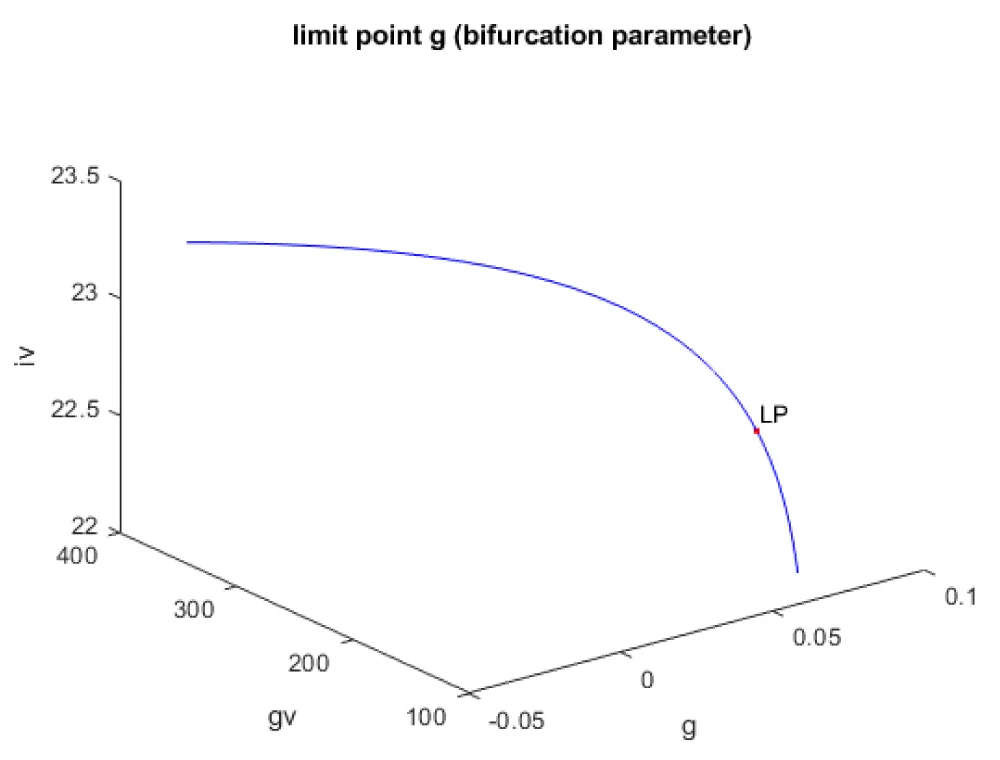
Figure 1a: Bifurcation diagram (g is the bifurcation parameter).
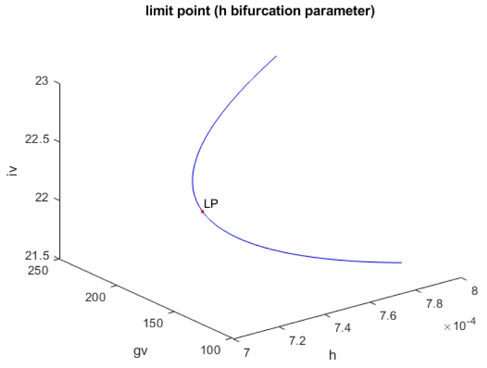
Figure 1b: Bifurcation diagram (h is the bifurcation parameter).
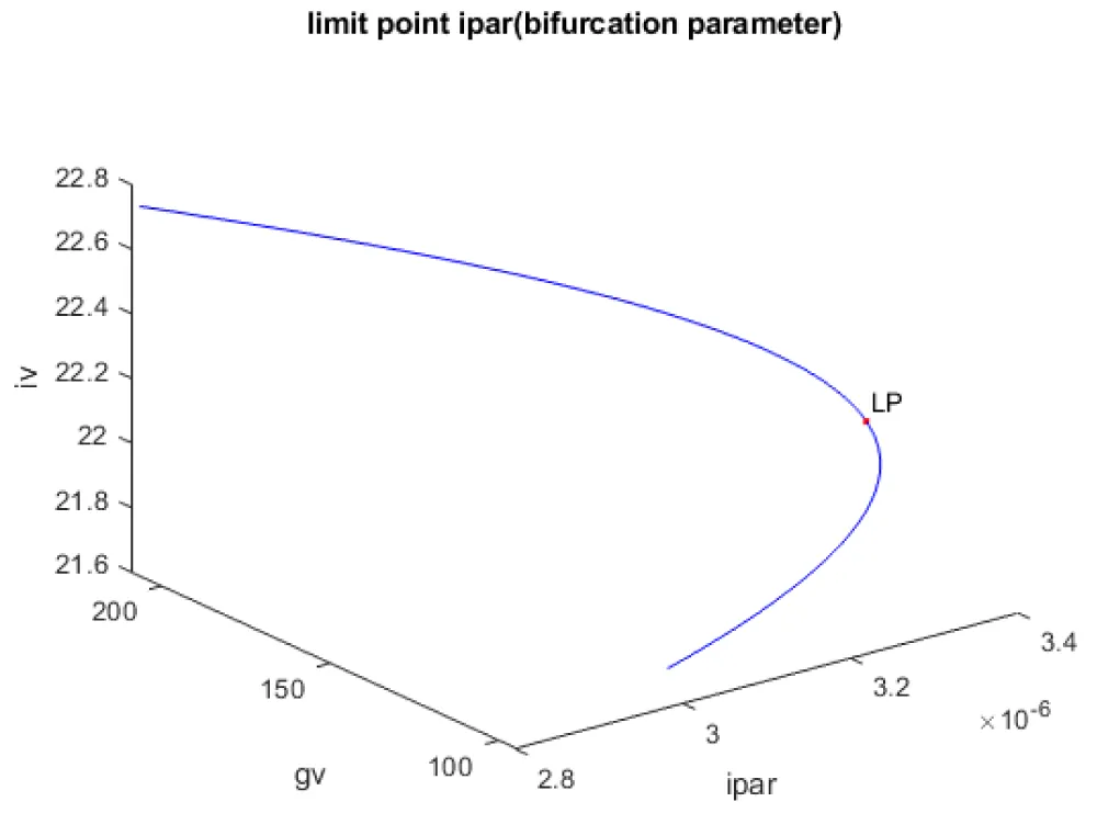
Figure 1c: Bifurcation diagram (ipar is the bifurcation parameter).
Hopf bifurcation points
A Hopf bifurcation point is a tipping point where a system that was behaving steadily suddenly starts to oscillate or cycle on its own, like a machine that begins to vibrate instead of staying still. Hopf Bifurcation points cause limit cycles. A limit cycle is a repeating pattern of behavior that a system naturally settles into over time, like a steady heartbeat or a clock that keeps ticking. The limit point (which causes multiple steady-state solutions from a singular point enables the Multiobjective nonlinear model predictive control calculations to converge to the Utopia point (the best possible solution) in the model. Kumari, et al. [20] show that when f was the bifurcation parameter, a Hopf point was found at (gv, iv, f) values of (82.030471 538.186016, 1.210489, 0.024461). This result is confirmed and reproduced (curve AB in Figure 1d). When f is modified to f(tan(f))/0.01 the Hopf bifurcation point disappears (curve CD in Figure 1d). The limit cycle caused by this Hopf bifurcation is shown in Figure 1e.
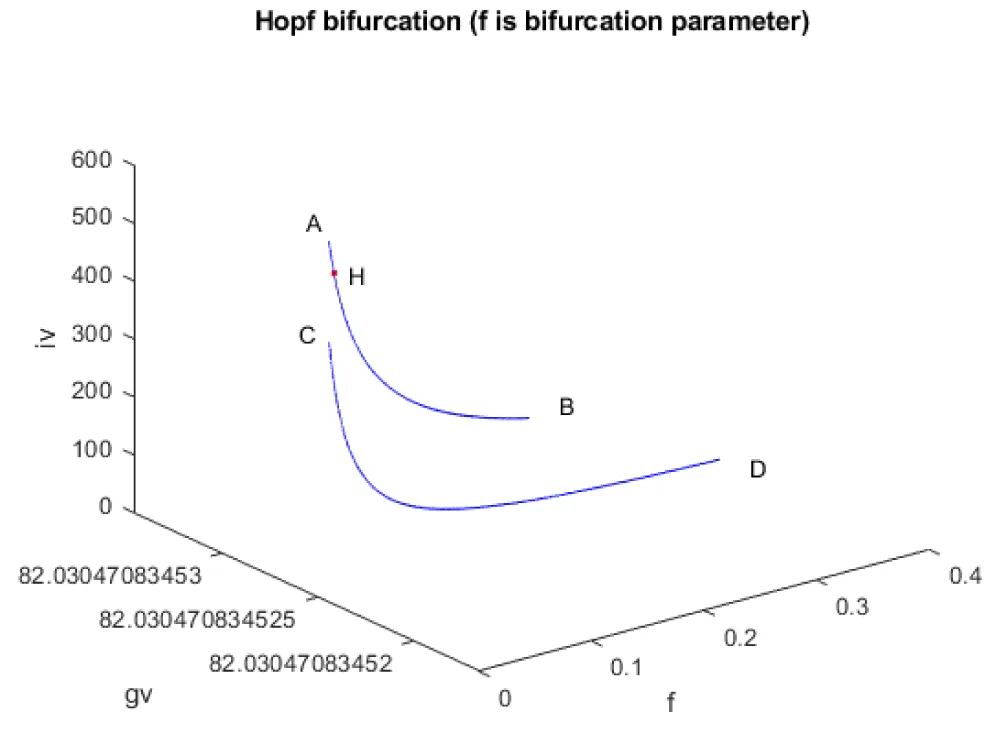
Figure 1d: Bifurcation diagram (f is the bifurcation parameter).
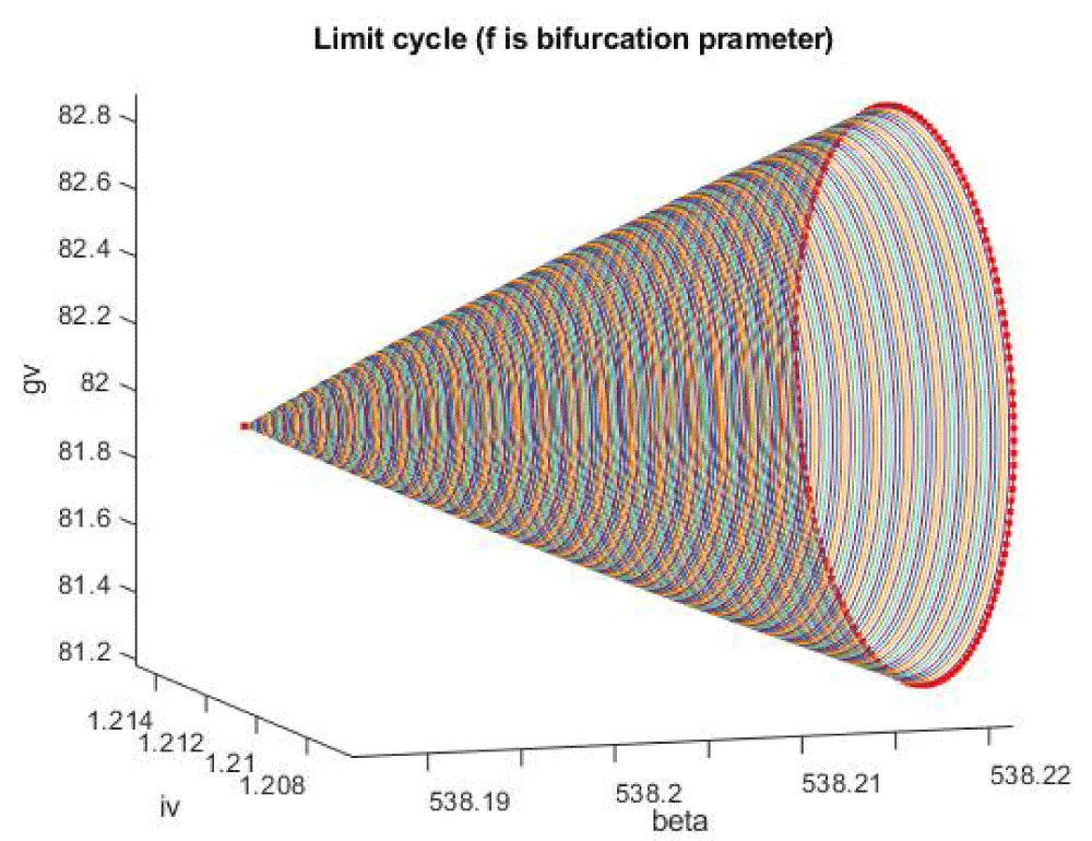
Figure 1e: Limit cycle caused by Hopf bifurcation (f is the bifurcation parameter).
Another Hopf bifurcation point was found when j was the bifurcation parameter at (gv, iv, j) values of (82.030471, 23.497933, 234.989285, 0.285128) (curve AB in Figure 1f). When f is modified to f(tan(f))/0.01, the Hopf bifurcation point disappears (curve CD in Figure 1f). The limit cycle caused by this Hopf bifurcation is shown in Figure 1g.
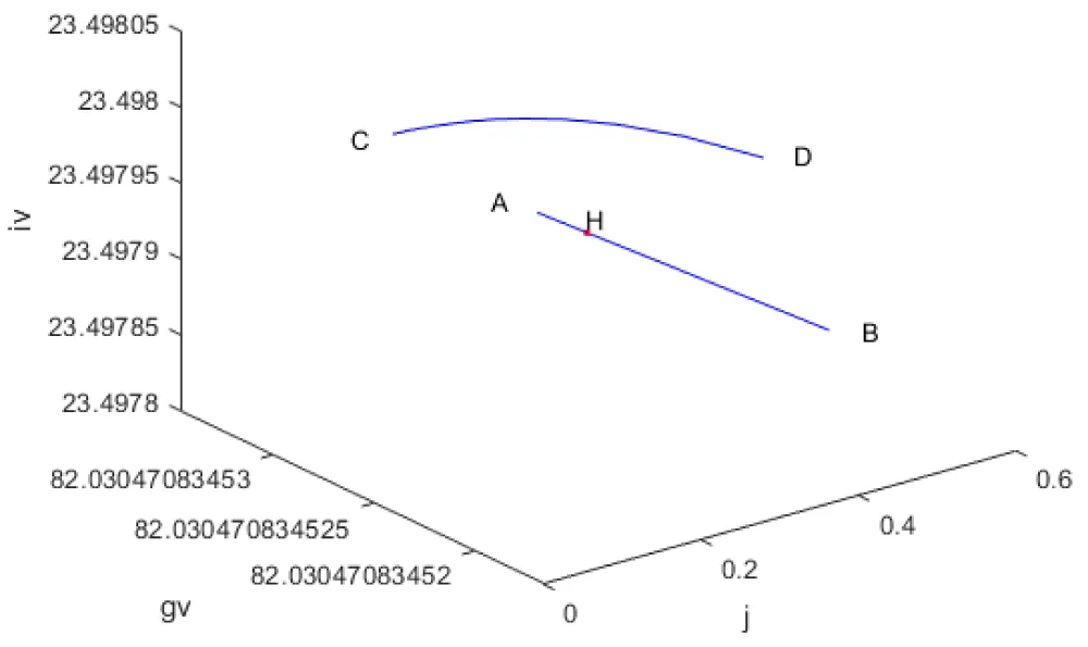
Figure 1f: Bifurcation diagram (j is the bifurcation parameter).
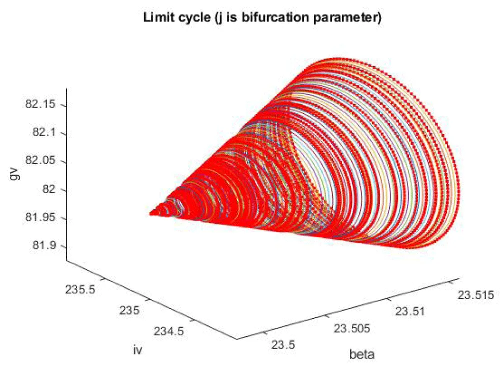
Figure 1g: Limit cycle caused by Hopf bifurcation (j is the bifurcation parameter).
The use of the tanh activation factor eliminated the limit cycle causing Hopf bifurcation, validating the analysis in Sridhar [30].
For the MNLMPC calculations in model 1, the values were maximized individually, and led to values of 2000.32903845 and 2003.55239404.
The overall optimal control problem will involve the minimization of
A cost function subject to the model’s governing equations. This led to a value of zero (the Utopia solution). A Utopia solution in multi-objective nonlinear model predictive control is an ideal operating point at which all goals are simultaneously perfectly optimized.
The MNLMPC value of the control variable, c1, was 5.735e-06. The various MNMPC figures are shown in Figures 2a-2d. The presence of the limit is beneficial because it allows the MNLMPC calculations to attain the Utopia solution, validating the analysis of Sridhar [36].
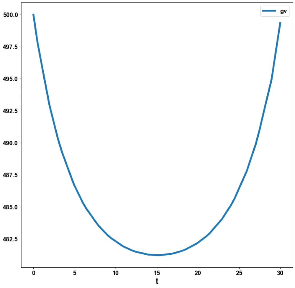
Figure 2a: MNLMPC (gv vs. t).
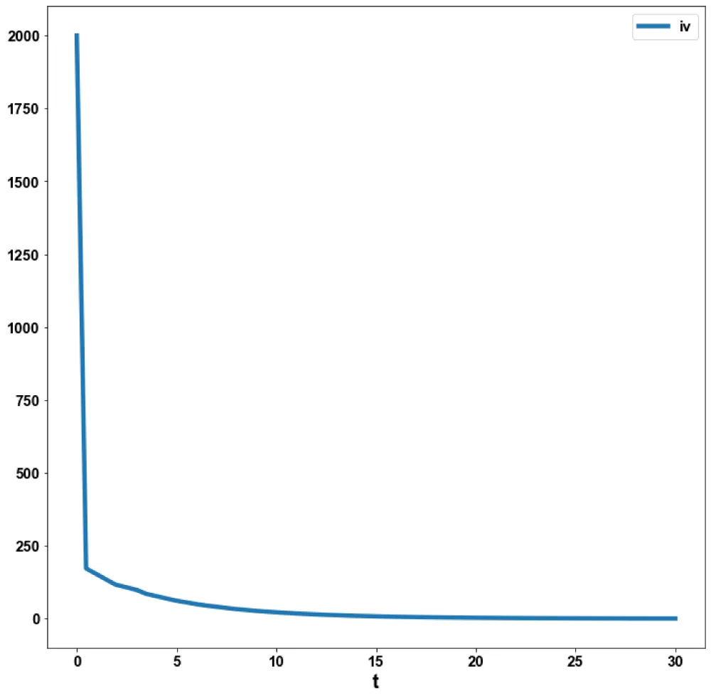
Figure 2b: MNLMPC (iv vs. t).
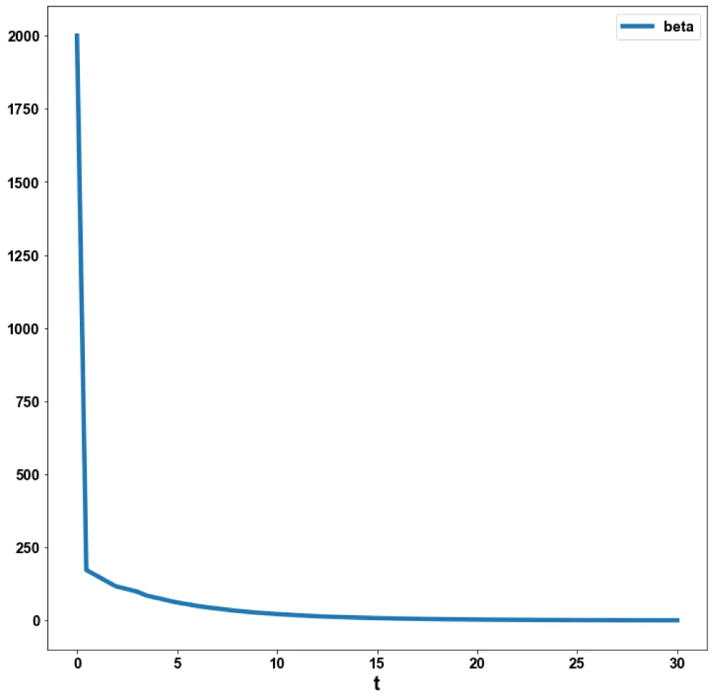
Figure 2c: MNLMPC (beta vs. t).
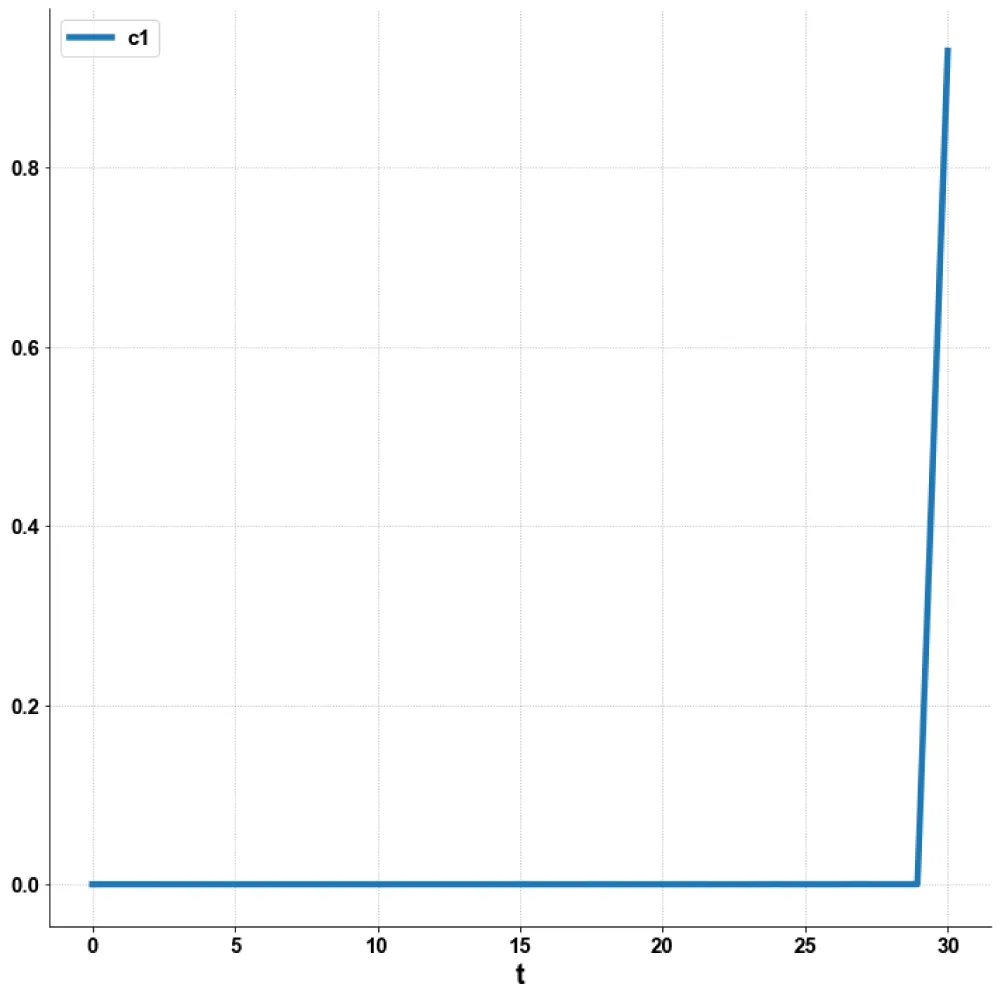
Figure 2d: MNLMPC (c1 vs. t).
Bifurcation analysis and multiobjective nonlinear control (MNLMPC) studies were performed on a Glucose-Insulin dynamic model. Hopf bifurcation points and limit points were detected. The Hopf bifurcation point, which causes an unwanted limit cycle, is eliminated using an activation factor involving the tanh function. The limit points (which cause multiple steady-state solutions from a singular point) are very beneficial because they enable the Multiobjective nonlinear model predictive control calculations to converge to the Utopia point (the best possible solution) in the models.
Data availability statement: All data used is presented in the paper
Conflict of interest: The author, Dr. Lakshmi N Sridhar, has no conflict of interest.
Dr. Sridhar thanks Dr. Carlos Ramirez for encouraging him to write single-author papers.
- Topp B, Promislow K, Devries G, Miura RM, Finegood DT. A model of B-cell mass, insulin, and glucose kinetics: pathways to diabetes. J Theor Biol. 2000;206(4):605. Available from: https://doi.org/10.1006/jtbi.2000.2150
- Lenbury Y, Ruktamatakul S, Amornsamarnkul S. Modeling insulin kinetics: responses to a single oral glucose administration or ambulatory-fed conditions. Biosystems. 2001;59(1):15–25. Available from: https://doi.org/10.1016/s0303-2647(00)00136-2
- Shanik MH, Xu Y, Skrha J, Dankner R, Zick Y, Roth J. Insulin resistance and hyperinsulinemia. Diabetes Care. 2008;31(Suppl 2):S262–S268. Available from: https://doi.org/10.2337/dc08-s264
- Han K, Kang H, Choi MY, Kim J, Lee M. Mathematical model of the glucose–insulin regulatory system: from the bursting electrical activity in pancreatic beta-cells to the glucose dynamics in the whole body. Phys Lett A. 2012;376(45):3150–3157. Available from: https://ui.adsabs.harvard.edu/abs/2012PhLA..376.3150H/abstract
- Lombarte M, Lupo M, Campetelli G, Basualdo M, Rigalli A. Mathematical model of glucose–insulin homeostasis in healthy rats. Math Biosci. 2013;245(2):269–277. Available from: https://doi.org/10.1016/j.mbs.2013.07.017
- Boutayeb W, Lamlili MEN, Boutayeb A, Derouich M. Mathematical modelling and simulation of B-cell mass, insulin and glucose dynamics: effect of genetic predisposition to diabetes. J Biomed Sci Eng. 2014;7(6):330–342. Available from: http://dx.doi.org/10.4236/jbise.2014.76035
- Ho CK, Sriram G, Dipple KM. Insulin sensitivity predictions in individuals with obesity and type II diabetes mellitus using a mathematical model of the insulin signal transduction pathway. Mol Genet Metab. 2016;119(3):288–292. Available from: https://doi.org/10.1016/j.ymgme.2016.09.007
- Brenner M, Abadi SEM, Balouchzadeh R, Lee HF, Ko HS, Johns M, et al. Estimation of insulin secretion, glucose uptake by tissues, and liver handling of glucose using a mathematical model of glucose-insulin homeostasis in lean and obese mice. Heliyon. 2017;3(6):e00310. Available from: https://doi.org/10.1016/j.heliyon.2017.e00310
- Mahata A, Mondal SP, Alam S, Roy B. Mathematical model of glucose-insulin regulatory system on diabetes mellitus in fuzzy and crisp environments. Ecol Genet Genom. 2017;2:25–34. Available from: https://www.researchgate.net/publication/309745279_Mathematical_model_of_glucose-insulin_regulatory_system_on_diabetes_mellitus_in_fuzzy_and_crisp_environment
- Shabestari PS, Panahi S, Hatef B, Jafari S, Sprott JC. A new chaotic model for glucose-insulin regulatory system. Chaos Solitons Fractals. 2018;112:44–51. Available from: https://doi.org/10.1016/j.chaos.2018.04.029
- Lombarte M, Lupo M, Brenda LF, Campetelli G, Marilia ARB, Basualdo M, et al. In vivo measurement of the rate constant of liver handling of glucose and glucose uptake by insulin-dependent tissues, using a mathematical model for glucose homeostasis in diabetic rats. J Theor Biol. 2018;439:205–215. Available from: https://doi.org/10.1016/j.jtbi.2017.12.001
- Kadota R, Sugita K, Uchida K, Yamada H, Yamashita M, Kimura H. A mathematical model of type 1 diabetes involving leptin effects on glucose metabolism. J Theor Biol. 2018;456:213–223. Available from: https://doi.org/10.1016/j.jtbi.2018.08.008
- Ali AH, Wiam B, Abdesslam B, Nora M. A mathematical model on the effect of growth hormone on glucose homeostasis. 2019. Available from: https://hal.science/hal-01909877v3/document
- Farman M, Saleem MU, Tabassum MF, Ahmad A, Ahmad MO. A linear control of composite model for glucose, insulin, and glucagon pump. Ain Shams Eng J. 2019;10(4):867–872. Available from: https://doi.org/10.1016/j.asej.2019.04.001
- Ibrahim MMA, Largajolli A, Karlsson MO, Kjellsson MC. The integrated glucose insulin minimal model: an improved version. Eur J Pharm Sci. 2019;134:7–19. Available from: https://doi.org/10.1016/j.ejps.2019.04.010
- Jamwal S, Ram B, Ranote R, Dharela S, Chauhan GS. New glucose oxidase-immobilized stimuli-responsive dextran nanoparticles for insulin delivery. Int J Biol Macromol. 2019;123:968–978. Available from: https://doi.org/10.1016/j.ijbiomac.2018.11.147
- Lopez-Zazueta C, Stavdahl Ø, Fougner AL. Simple nonlinear models for glucose-insulin dynamics: application to intraperitoneal insulin infusion. IFAC-PapersOnLine. 2019;52(26):219–224. Available from: https://www.researchgate.net/publication/338191556_Simple_Nonlinear_Models_for_Glucose-Insulin_Dynamics_Application_to_Intraperitoneal_Insulin_Infusion
- Loppini A, Chiodo L. Biophysical modeling of beta-cells networks: realistic architectures and heterogeneity effects. Biophys Chem. 2019;254:106247.
- Stamper IJ, Wang X. Integrated multiscale mathematical modeling of insulin secretion reveals the role of islet network integrity for proper oscillatory glucose-dose response. J Theor Biol. 2019;475:1–24. Available from: https://doi.org/10.1016/j.jtbi.2019.05.007
- Kumari P, Singh S, Singh HP. Bifurcation and stability analysis of glucose-insulin regulatory system in the presence of beta-cells. Iran J Sci Technol Trans A Sci. 2021. Available from: https://doi.org/10.1007/S40995-021-01152-X
- Dhooge A, Govaerts W, Kuznetsov AY. MATCONT: a MATLAB package for numerical bifurcation analysis of ordinary differential equations. ACM Trans Math Softw. 2003;29(2):141–164. Available from: https://lab.semi.ac.cn/download/0.28315849875964405.pdf
- Dhooge A, Govaerts W, Kuznetsov AY, Mestrom W, Riet AM. CL_MATCONT: a continuation toolbox in MATLAB. 2004. Available from: https://doi.org/10.1145/952532.952567
- Kuznetsov YA. Elements of applied bifurcation theory. New York: Springer; 1998. Available from: https://www.ma.imperial.ac.uk/~dturaev/kuznetsov.pdf
- Kuznetsov YA. Five lectures on numerical bifurcation analysis. Utrecht (Netherlands): Utrecht University; 2009.
- Govaerts WJF. Numerical methods for bifurcations of dynamical equilibria. Philadelphia: SIAM; 2000.
- Dubey SR, Singh SK, Chaudhuri BB. Activation functions in deep learning: a comprehensive survey and benchmark. Neurocomputing. 2022;503:92–108. Available from: https://doi.org/10.1016/j.neucom.2022.06.111
- Kamalov AF, Nazir M, Safaraliev AK, Cherukuri R, Zgheib R. Comparative analysis of activation functions in neural networks. In: Proceedings of the 28th IEEE International Conference on Electronics, Circuits, and Systems (ICECS); 2021; Dubai, United Arab Emirates. p. 1–6. Available from: https://ieeexplore.ieee.org/document/9665646
- Szandała T. Review and comparison of commonly used activation functions for deep neural networks. arXiv. 2020. Available from: https://doi.org/10.1007/978-981-15-5495-7
- Sridhar LN. Bifurcation analysis and optimal control of the tumor–macrophage interactions. Biomed J Sci Tech Res. 2023;53(5):MS ID 008470. Available from: https://biomedres.us/pdfs/BJSTR.MS.ID.008470.pdf
- Sridhar LN. Elimination of oscillation causing Hopf bifurcations in engineering problems. J Appl Math. 2024;2(4):1826. Available from: https://ojs.acad-pub.com/index.php/JAM/article/view/1826
- Flores-Tlacuahuac A, Morales P, Rivera Toledo M. Multiobjective nonlinear model predictive control of a class of chemical reactors. Ind Eng Chem Res. 2012;51:5891–5899. Available from: https://doi.org/10.1021/ie201742e
- Hart WE, Laird CD, Watson JP, Woodruff DL, Hackebeil GA, Nicholson BL, et al. Pyomo: optimization modeling in Python. 2nd ed. New York: Springer; 2021. Available from: https://link.springer.com/book/10.1007/978-3-030-68928-5
- Wächter A, Biegler L. On the implementation of an interior-point filter line-search algorithm for large-scale nonlinear programming. Math Program. 2006;106:25–57. Available from: https://doi.org/10.1007/s10107-004-0559-y
- Tawarmalani M, Sahinidis NV. A polyhedral branch-and-cut approach to global optimization. Math Program. 2005;103(2):225–249. Available from: https://doi.org/10.1007/s10107-005-0581-8
- Sridhar LN. Coupling bifurcation analysis and multiobjective nonlinear model predictive control. Austin Chem Eng. 2024;10(3):1107. Available from: https://austinpublishinggroup.com/chemical-engineering/fulltext/ace-v11-id1107.pdf
- Upreti SR. Optimal control for chemical engineers. 1st ed. Boca Raton: Taylor & Francis; 2013. Available from: https://doi.org/10.1201/b13045